In this section we will discuss the status of the HET facility and each instrument and any limitation to configurations that occurred during the period.
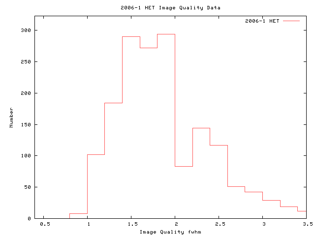
The following FWHM image quality statistics were taken from the LRS pre-imaging statistics and FIF acquisition guider for science operations in the night report. These are true FWHM measures using the same software on both the FIF acquisition guider and the LRS pre-images.
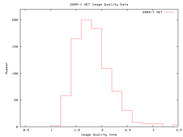
For comparison here is the LRS pre-imaging quality for the same period of 2004
Here are the DIMM values reported in the night report.

Month by Month Summary
The following table gives the observing statistics for each month. The second column gives the fraction of the month that was spent attempting science (as opposed to engineering or instrument commissioning). Science time is defined to begin at 18 degree twilight or the first science target. Science time is defined to end at 18 degree twilight or the last science target. The fourth column gives the fraction of the possible science time (A) lost due to weather. The fifth through seventh columns give the amount of remaining science time (after removing weather losses) not spent attempting science targets. Please note that the first stack of the night often occurs before 18 degree twilight.
| Month | A:Fraction of the Time that was Possible Science | B:Average Night Length | C:Fraction of Total Science Time Lost due to Weather | D:Fraction of Actual Science Time Spent with Shutter Open | D:Fraction of Actual Science Time Lost due to Overhead | E:Fraction of Actual Science Time Lost due to Calibrations | D:Fraction of Actual Science Time Lost due to Alignment | F:Fraction of Actual Science Time Lost due to Problems | Fraction of Actual Science Time Not accounted for or Lost |
|---|---|---|---|---|---|---|---|---|---|
| December | 0.992 | 10.94 | 0.22 | 0.52 | 0.36 | 0.01 | 0.04 | 0.06 | 0.02 |
The last column accounts for all of the minutes lost or not used. Some of this time is accounting errors, some is time not charged to any program due to operations inefficiency and some is due to uncharged overheads from observations that did not result in a fits file.
Details on Nightly cloud cover based on the TO's observations of the sky reported 3 times a night in the night report.:
| Month | Fraction of the Nights that were Clear | Fraction of the Nights that were Mostly Clear | Fraction of the Nights that were Partly Cloudy | Fraction of the Nights that were Mostly Cloudy | Fraction of the Nights that were Cloudy |
|---|---|---|---|---|---|
| December | 0.26 | 0.32 | 0.19 | 0.07 | 0.16 |
Please note that the HET could be closed due to humidity, smoke or high dust count and still have a "Clear" statistic in the night report.
The following tables give a break down of all attempted visits as well as the category that each falls into.
| Charged exposures | ||
|---|---|---|
| Number of Times | Shutter Open (Hours) | Type |
| 528 | 85.1 | A - Acceptable |
| 25 | 5.6 | B - Acceptable but Border line conditions |
| 162 | 24.4 | 4 - Priority 4 visits (does not include 1/2 charge) |
| 0 | 0.0 | Q - charged but PI error |
| 0 | 0.0 | C - Acceptable by RA but PI rejects |
| Uncharged exposures | ||
|---|---|---|
| Number of Times | Shutter Open (Hours) | Type |
| 18 | 2.8 | I - Targets observed under otherwise idle conditions |
| 7 | 1.4 | E - Rejected by RA for Equipment Failure |
| 7 | 1.4 | H - Rejected for Human failure |
| 14 | 2.0 | W - Rejected by RA for Weather |
| 1 | 0.1 | P - Rejected by PI and confirmed by RA |
| 3 | 0.0 | N - Rejected due to unknown cause |
So this is a total of 7.7 hours of uncharged spectra with an additional possible 5.6 hours of spectra that may be rejected.
The following overhead statistics include slew, setup, readout and refocus between exposures (if there are multiple exposures per visit). In the summary page for each program the average setup time is calculated. The table below gives the average setup time for each instrument PER VISIT and the average and maximum COMPLETED science exposures and visits.
The "Exposure" is defined by when the CCD opens and closes. A "Visit" is the requested total CCD shutter open time during a track and might be made up of several "Exposures". "Visit" as defined here contains no overhead. To calculate one type of observing efficiency metric one might divide the "Visit" by the sum of "Visit" + "Overhead".
The average overhead per actual visit is the overhead for each acceptable priority 0-3 (not borderline, and with overheads > 4 minutes to avoid 2nd half of exposures with unrealisticly low overheads) science target. This number reflects how quickly we can move from object to object on average for each instrument, however, this statistic tends to weight the overhead for programs with large number of targets such as planet search programs.
The average overhead per requested visit is the total charged overhead per requested priority 0-3 visit averaged per program. To get this value we average the average overhead for each program as presented in the program status web pages. The average overhead per visit can be inflated by extra overhead charged for PI mistakes (such as bad finding charts or no targets found at sky detection limits) or for incomplete visits e.g. 2 visits of 1800s are done instead of 1 visit with a CRsplit of 2. The average overhead per visit can be deflated by the 15 minute cap applied to the HRS and MRS. This method tends to weight the overhead to programs with few targets and bad requested visit lengths, ie. very close to the track length.
| Instrument | Avg Overhead per Actual Visit(min) | Avg Overhead per Requested Visit(min) | Avg Exposure (sec) | Median Exposure (sec) | Max Exposure (sec) | Avg Visit (sec) | Median Visit (sec) | Max Visit (sec) |
|---|---|---|---|---|---|---|---|---|
| LRS | 14.4 | 14.2 | 837.2 | 900 | 1800 | 1500.7 | 1800 | 2700 |
| HRS | 10.2 | 11.7 | 550.4 | 580 | 2070 | 783.8 | 600 | 4140 |
| MRS | 12.1 | 12.6 | 708.6 | 600 | 1650 | 1156.2 | 710 | 1800 |
NOTE: AS OF 2003-3 THE SETUP TIME FOR AN ATTEMPTED MRS OR HRS TARGET IS CAPPED AT 15 MINUTES. AS OF 2004-3 THE SETUP TIME FOR AN ATTEMPTED LRS TARGET IS CAPPED AT 20 MINUTES.
The overhead statistics can be shortened by multiple setups (each one counted as a separate visit) while on the same target as is the case for planet search programs. The overhead statistics can be lengthened by having multiple tracks that add up to a single htopx visit as can happen for very long tracks where each attempt might only yield a half visit.
A way to improve the overhead accumulated for programs with long exposure times is to add double the above overhead to the requested visit length and make sure that time is shorter than the actual track length. This avoids the RA having to split requested visits between several different tracks.
During this period we have had some trouble with LRS setups which have turned out to be training issues.
The following links give the summary for each institution and its programs.
The resulting table will give (for each program) the total number of targets
in the queue and the number completed, the CCD shutter open
hours, average overhead for that program, and the TAC allocated time.
This usually will be the best
metric for judging completeness but there are times when a PI will tell
us that a target is "done" before the total number of visits is complete.
This is how each institution has allocated its time by priority.
Observing Programs Status
Program comments:
UT06-1-001: (Kilic) priority 1-2, g2
UT06-1-003: (Benedict) priority 1-3 HRS
UT06-1-004: (Hoflich) priority 0-2 LRS TOO
UT06-1-005: (Hoflich) priority 1-3 LRS ToO
UT06-1-006: (Shetrone) priority 1-3 , HRS
UT06-1-007: (Sobeck) priority 1-3 HRS, P1 complete
UT06-1-008: (Robinson) priority 0 , TOO
UT06-1-009: (Wheeler) priority 0 , TOO
UT06-1-010: (Cochran) priority 1-4 , HRS
UT06-1-011: (Kormendy) priority 1-3 LRS g2
UT06-1-012: (Quimby) priority 0-2 LRS g1
UT06-1-014: (Wittenmyer) priority 1-4 HRS
UT06-1-015: (Allende-Prieto) priority 2-4 HRS, P2-3 complete
UT06-1-017: (Allende-Prieto) daysky, HRS
UT06-1-019: (Benedict) priority 1-3 HRS, P1 complete
UT06-1-020: (Benedict) priority 0-1 HRS
UT06-1-021: (Maund) priority 0 LRS g2
Program comments:
PSU06-1-001: (Wolszczan) priority 2-4 HRS
PSU06-1-002: (Wolszczan) priority 2-4 HRS,
PSU06-1-003: (Budaj) priority 2 HRS, program complete
PSU06-1-005: (Gronwall) priority 2-4, no Phase II
PSU06-1-006: (Fox) priority 0-1 , no phase II
PSU06-1-007: (Schneider) priority 1-2 , SN program run by STA06-1-001
PSU06-1-008: (Schneider) priority 2, no phase II
PSU06-1-009: (Herrmann) priority 0-1,3 MRS
PSU06-1-010: (Luhman) priority 1-2 LRS g3, Program complete
PSU06-1-011: (Eracleous) priority 1-2,4, LRS g3
PSU06-1-012: (Eracleous) priority 1, LRS g1
PSU06-1-014: (Richards) priority 4 LRS g3
PSU06-1-015: (Brown) priority 1-3 MRS, no phase II
PSU06-1-016: (Retter) priority 4 LRS g1
PSU06-1-017: (Wade) priority 1-3 MRS, P1-2 complete
PSU06-1-018: (Wade) priority 3 MRS
PSU06-1-019: (Brandt) priority 2,4, no phase II
PSU06-1-020: (Brandt) priority 1-3 LRS g2
PSU06-1-101: (Williams) priority 1 no Phase II recieved
PSU06-1-102: (Ge) priority 0 HRS
Program comments:
STA06-1-001: (Romani/Masao) priority 0-2 LRS g1 TOO, P0 complete, priorities combined from other institutions
STA06-1-002: (Romani/Michelson) priority 1-3 LRS g1, P1 complete
STA06-1-003: (Abel) priority 1-2 LRS g2 and HRS, P1 complete
Program comments:
M06-1-001: (Feulner) priority 3 LRS g1, MOS
M06-1-002: (Hopp) priority 0,2 SN program run by STA06-1-001
M06-1-003: (Bender) priority 1-2 LRS g2
M06-1-004: (Saglia) priority 1-3 LRS e2,
Program comments:
G06-1-001: (Kollatschny) priority 2-3 LRS g2
G06-1-003: (Zetzl) priority 1-3 LRS g2
G06-1-004: (Homeier) priority 2-3 HRS
G06-1-005: (Unknown) priority 1-2 LRS SN program run by STA06-1-001
Institution Status
| Time Allocation by Institution (hours) | |||||
|---|---|---|---|---|---|
| Institution | Priority 0 | Priority 1 | Priority 2 | Priority 3 | Priority 4 |
| PSU | 10.910 (5%) | 34.970 (17%) | 40.190 (20%) | 38.050 (19%) | 80.820 (39%) |
| UT | 15.000 (5%) | 73.000 (24%) | 84.000 (28%) | 85.000 (28%) | 46.000 (15%) |
| Stanford | 3.000 (9%) | 8.000 (24%) | 11.000 (33%) | 11.000 (33%) | 0.000(0%) |
| Munich | 2.000 (6%) | 8.000 (25%) | 12.000 (38%) | 10.000 (3%) | 0.000 (0%) |
| Goetting | 0.000 (0%) | 5.000 (22%) | 8.500 (37%) | 9.700 (42%) | 0.000 (0%) |
| SALT | 0.000 | 0.000 | 0.000 | 0.000 | 0.000 |
| DDT | 0.000 | 0.000 | 0.000 | 0.000 | 0.000 |
The following is a summary of the Acceptable CCD shutter time for each institution based on our htopx data base. It does not include any overhead. And does not weight based on any priority scheme (ie. priority 4 are counted at full cost).
| CCD shutter Open by Institution (hours) | ||||
|---|---|---|---|---|
| -TOTAL- | Used | % of All | ||
| PSU | 21.701 | 18.5 | ||
| UT | 65.419 | 55.8 | ||
| Stanford | 23.167 | 19.7 | ||
| Munich | 4.133 | 3.5 | ||
| Goetting | 2.917 | 2.5 | ||
| NOAO | 35.253 | -- | ||
| SALT | 0.000 | -- | ||
| DDT | 0.000 | -- | ||
NOTE: At the present time the Stanford lead SN project has not allocated any time to any of the partners so the entire allocation is currently charged to Stanford.
The following is a summary of the total charged time for each institution based on our htopx data base (for shutter open) and night reports (for overhead). It includes shutter open time (weighting priority four by half) and overhead.
| Time Charged by Institution (hours) | |||||
|---|---|---|---|---|---|
| -INST- | Used THIS PERIOD | % of All THIS PERIOD | - % ALLOCATION TO DATE- | ||
| PSU | 34.4 | 19.4% | 29.93% | ||
| UT | 91.7 | 51.8% | 54.41% | ||
| Stanford | 40.0 | 22.6% | 6.65% | ||
| Munich | 6.6 | 3.7% | 4.49% | ||
| Goetting | 4.4 | 2.5% | 4.50% | ||
| NOAO | N/A | -- | -- | ||
| SALT | 0.00 | -- | -- | ||
| DDT | 0.00 | -- | -- | ||
Total to Date starting from Oct 1999.
Priority weighting for P4 began in the 2003-2 period.
NOTE: At the present time the Stanford lead SN project has not allocated any time to any of the partners so the entire allocation is currently charged to Stanford.
| UT06-1 | ||
|---|---|---|
| Rank | Program | Constraints |
| 1 | UT06-1-010 HD_45350, GJ_270, HD_51295 | HRS, EE50 < 2.0, Vsky > 19.0 |
| 2 | UT06-1-003 HD33636, HD12661 | HRS, EE50 < 3.0, Vsky > 19.0 |
| PSU06-1 | ||
|---|---|---|
| Rank | Program | Constraints |
| 1 | PSU06-1-009 M101_PN | MRS, EE50 < 2.5, Vsky > 20.4 |
| 2 | PSU06-1-011 4C_36.18 | LRS G3 EE50 < 2.0, Vsky > 20.4 |
| STA06-1 | ||
|---|---|---|
| Rank | Program | Constraints |
| 1 | STA06-1-001 SN_gal | LRS EE50 < 1.8, Vsky > 20.3 |
| 2 | STA06-1-003 Sextans_98 | HRS EE50 < 1.8, Vsky > 20.6 |
| M06-1 | ||
|---|---|---|
| Rank | Program | Constraints |
| 1 | M06-1-004 NGC3623, NGC4314, NGC4321 | LRS e2 EE50 < 2.0, Vsky > 21.3, |
| 2 | M06-1-001 MUNICS_S2F5_Setup2 | LRS g1 MOS EE50 < 2.0, Vsky > 21.3, |
| G06-1 | ||
|---|---|---|
| Rank | Program | Constraints |
| 2 | G06-1-004 HS1253+1033, HS1443+2934 | LRS G2 EE50 < 4.0, Vsky > 18.0 |
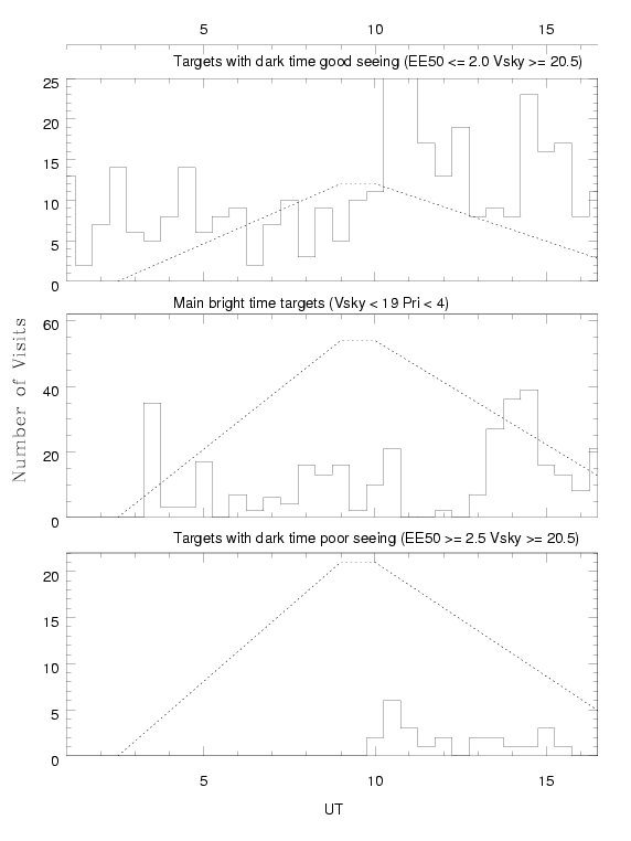
The following histogram shows some of the extrema in observing conditions: good seeing dark time, bright time and bad seeing dark time. A line has been drawn at the expected number of hour long visits that we hope to achieve in each hour bin.
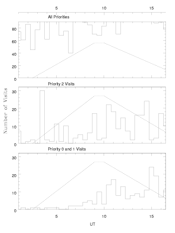
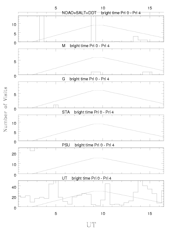
The following histogram shows the bright time priority 0-3 contribution from each partner. The dashed line is a rough estimate of the number of hour long visits one could complete during the remainder of the period.
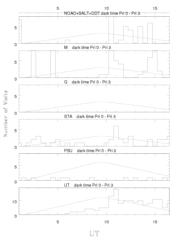
The following histogram shows the dark time priority 0-3 contribution from each partner. The dashed line is a rough estimate of the number of hour long visits one could complete during the remainder of the period.
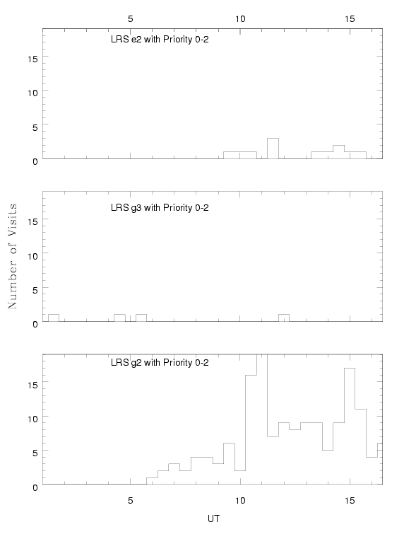
The following histogram shows the use of LRS_g2 vs. LRS_g3 and LRS_e2 for priority 0-2 programs in this period.
From the above plots I have determined that: