HET Hex Burst Studies - HBT Users Manual

The HET hexburst procedure provides us with a method of identifying problem mirrors in the array. The HEFI camera is used to image the stacked array at best focus. Offsets are then sent to the array that shift each mirror by some amount. The resulting image obtained with the HEFI camera is then a series of point sources distributed in a pattern that mimics the shape of the HET mirror array. Each source in this HEFI picture represents the image formed by an individual mirror. An example of such an image is shown below in Figure 1. By identifying the mirror producing each image, and by measuring certain properties of each image, we can produce a useful record of mirror properties. This is the job of the HBT code. A record of image properties kept over time can be used by Jerry Martin and the rest of the day crew to identify mirrors that need cleaning/aluminizing, mirrors that have large focus offsets relative to the array as a whole, or mirrors that produce distorted images due possibly to support problems.

Since a lot of things changed over the course of developing HBT, the present procedures for reducing hexburst data are a little convoluted. Hopefully, this manual will direct us along the path towards a streamlined analysis approach. Initially, we simply took a series of HEFI images at different focus settings. The job of HBT was to allow the reducer to easily identify the mirrors in each HEFI image (i.e. each focus value), measure image parameters for each mirror, identify the best focus setting for each mirror, and finally, summarize all of the results in a web document. Later, we began taking images with the HEFI lamp set on a high and low setting. Moreover, we took multiple sets of images at each focus. To handle this change, a pre-reduction code was developed called HBTPREP. This routine handles the registration of images in each focus/lamp group. In reality, it sets up the input script needed to perform this registration and stacking procedure inside IRAF. After we have stacked the hexburst images with HBTPREP and IRAF, we run HBT.

For this manual, I will often show the prompts displayed by HBT or HBTPREP. To denote the user-supplied responses, I will highlight them in RED.

Notes on taking hexburst images.

Below I list a few points on name conventions for hexburst image files. The RA can run a script that renames all images afetr the the TO completes each set.

Name bias frames: 
   bst_bias0001.fits 
   bst_bias0002.fits 
   bst_bias0003.fits 
   etc...

Typical hex burst image name: 
    tr_f=-200_lo_05.fits
     1   2    3  4

 1: Inidcates if image is Tracker Right (=r) or Tracker Left (=l) 
 
 2: The relative focus value, with sign included. Please preceed 
    the integer focus value with "f=" in the file name. 

 3: Indicates whether lamp setting is lo or hi. This is now not needed
    since we ONLY use lo settings. To avoid software changes and keep 
    a historically smooth archive we include this part of the name now. 

 4: A running image name (automatically assigned when running HEFI 
    camera). 

OTHER NOTES:
  A) If you have taken a focus=0 image (and used "f=0" in the 
     image names), and then return to do another focus=0 image, 
     do not use "f=0" again! This will just over-write the first 
     set. Use "f=+10", as this small offset will make no difference 
     in the analysis. 

Finally, the easiest way to get the image names set properly is to have the RA run a script to perform the renaming after each set of hefi images at a focus position have been collected by the TO. Here is a typical renaming script:

#
mv h0001.fits tr_f=1890_lo_01.fits
mv h0002.fits tr_f=1890_lo_02.fits
mv h0003.fits tr_f=1890_lo_03.fits
mv h0004.fits tr_f=1890_lo_04.fits
mv h0005.fits tr_f=1890_lo_05.fits
mv h0006.fits tr_f=1890_lo_06.fits
mv h0007.fits tr_f=1890_lo_07.fits
mv h0008.fits tr_f=1890_lo_08.fits
mv h0009.fits tr_f=1890_lo_09.fits
mv h0010.fits tr_f=1890_lo_10.fits
mv h0011.fits tr_f=1890_lo_11.fits
mv h0012.fits tr_f=1890_lo_12.fits
mv h0013.fits tr_f=1890_lo_13.fits
mv h0014.fits tr_f=1890_lo_14.fits
mv h0015.fits tr_f=1890_lo_15.fits

A Brief Overview of the Current Process

A major overhaul of the procedures used in reducing hexburst data was performed in Spring 2006. Some of these new steps are not yet described in this web document. I provide a terse outline of the current process below.

Codes reside at:
/home/banzai/sco/projects/het_sco/src/sco_het_code/hbtcodes
hbt/  hbt_combine/  hbtfinal/  hbtprep/  hbtweb/

Also, on mcs: 
/home/mcs/sco/projects/het_sco/src/sco_het_code/hbtcodes
hbt/  hbt_combine/  hbtfinal/  hbtprep/  hbtweb/  README.hbt  refoc/


A rough outline for using hbt codes:

1) Use hbt to gather info on what dataset are available.
   Pull over desired data sets for reduction.

2) Use iraf to bias correct HEFI image.

3) Run hbtprep to prepare iraf scripts for stacking image.
   Use iraf to make the stacks. Use renaming scripts made by
   hbtprep to rename the stacked image.

4) Run HBT to identify the mirrors at each focus position.

  NOTE:
  Here is where all of the big changes of Spring 2006 have a
  big effect. I used to do the full analysis in HBT (i.e. fitting
  focus curves, etc). HBT made (and still makes!) web pages
  summarizing the analysis. I would reduce tracker left,right
  images sets separately. The code called hbt_combine was used
  to combine such left,right sets and compare results. Basically
  just produce a few gif plots.

  ====> Now I use hbt just through the mirror identification
        step.

5) The hbtfinal code now stacks the inidividual mirror images
   at each focus set. This is done using file made by the hbtprep
   and hbt runs. Refined image parameters are computed, and the
   focus curve fitting is done in hbtfinal. The plots and registered
   (fits) stamps, as well as gif files of "best focus" images are
   archived by hbtfinal.

6) The hbtweb code (still being developed as of July 2007) fully
   archives the run. It presently produces ASCII data tables for
   mirrors analyzed in the tracker left,right analyses. It will
   soon produce a set of summary web pages comparable to that made
   with hbt alone, but of course this new analysis is based on
   more precisely stacked image sets.

Running HBT-related Codes on Solaris Monitors

The HBT-related programs often rely on a fast graphics capability. This is not possible on the Solaris machines (mcs and ion) available in the HET control room. The solution is to run the code on one of our fast linux boxes using one of the availble Solaris monitors. Ordinarily, the linux machine will be beta. Here is how to do it if you are working from ion:

On ion:
xhost +beta

On beta (after you have ssh'd in):
setenv DISPLAY ion:0.0

Initial Setup Steps

Running any of the HBT-related software packages requires some supporting files that, if present, make operation more streamlined. You need not worry about them here. I have prepared a script that will build these files in the directory you working in. Just type on your command line:

 hbt_ready_linux     On a linux machine 
 hbt_ready_solaris    On a Solaris machine 

Running HBT to Prepare for the Reduction

sco@ion:T> HBT
Jump directly to HBT-related tasks? (Y/N): Y

==================================================== 
HBT-related tasks: 
 1) Read and manipulate tip files
 2) Find hexburst data sets
 3) Summarize and prepare a hexburst for reduction
 4) Build a script to reconstruct a web page

99) Leave this section of HBT 
Enter desired task code (99): 2

Are you running on new mcs? (Y/N): Y

20050216
20050217
20050307
20050319
20050404
20050616
20050617
20050701
20050715
20050827
20051011
20051012

 ======================================================
  See the local file called "hexburst_data.list" for a
  summary of all hexburst data sest available now.
 ======================================================

After running task 2, you can view the local file called hexburst_data.list to see what data are available. You can quickly determine how many images are available in a data set (N_images), how many of those images are compressed (N_compressed), and how many HEFI bias frames are avalible for that set (N_bias). An example of such a file is shown below.

Directory    N_images  N_compressed  N_bias
20050216       160          160         0
20051012       180          180         0
20051022       190          195         5
20051118       603          623        20
20051124       660          680        20
20051225       660          680        20
20051231       570          590        20
20060120       480          500        20
20060131       676          696        20

Next, you can run task 3 and get a more detailed summary of the available hexburst data. Here, a file called hexprep.out is created. Here is an example of such a file:

Ntot   = total number of hexburst images
N_l    = number of tracker_left images
N_r    = number of tracker_right images
N_lo   = number of low lamp images
N_hi   = number of high lamp images
Fmin   = minimum focus value
Fmax   = maximum focus value

Note: C indicates the image data are compressed

Directory  Ntot     N_l  N_r    N_lo N_hi     Fmin  Fmax

 20050216   160      80   80      80   80    -600    600    C
 20050217   190      80  110     100   90    -800   1000    C
 20050307   200     100  100     100  100       0   2400    C
 20050319   200     100  100     100  100       0   2400    C
 20050404   170      80   90      85   85   -2300      0    C
 20050423   100       0  100      50   50    -600   1000    C
 20050502   100       0  100      50   50    -600   1000    C
 20050616   200      95  105     105   95   -1000    600    C
 20050617   220     110  110     110  110   -1200    800    C
 20050701   205     100  105     100  100    -600   1000    C

Note that option 3 can actually perform two tasks. In the first case, you can produce a table like that above (job choice 1). By selecting job choise 2, you can set up for reducing a specific hexburst set. You will be queried for the name of the hexburst directory (i.e. 20050502). A script is created (called "MAKE_1.SCRIPT") that can be used to pull over the neccassary images for a reduction and store them in a convenient directory tree structure.

Note that at this time, it is very important that you use one of the hexburst data summary files (above) to determine if the data files are compressed or not. If the files are compressed, then you should use the unix uncompress command in the guider directory in question. This must be done prior to completing a run of job choice 2 in option 3, otherwise the images names will not be interpretted correctly. Here is an example of how you might do this:

> cd /data1/mcs/guider/20050502
> uncompress *.Z

A SPECIAL NOTE: If the hexburst images were named properly, then the option 3 step explained above will automatically perform steps need for HBTPREP. The tracker-left and tracker-right images will be written to separate reduction directories (called Tl_lo and Tr_lo respectively). These directories will contain the hbtprep.in files that you will need to run HBTPREP. Also, the bias frames will be deposited in a local directory called zero.

Running HBTPREP

Our first job (after transferring the hexburst data set to our reduction machine) is to subtract the HEFI bias pattern from each HEFI image, and then combine the images sets taken at each focus setting and lamp setting. The following procedure describes what is being done as of July 2007.

If the bias frames are available for your hexburst set, then the first data reduction task will be the construction of a mean bias frame, and the subtraction of that mean frame from all of your hexburst images. Some of these steps will be done with IRAF. Normally, we will maintain a directory called iraf that will be dedicated to hexburst reductions. You will normally just go to the working hexburst iraf directory and type "cl" to start up iraf.

Step 0: Confirm bias images are present. 
In many of the early hexburst data sets no bias frame images 
were collected. These images should have the name 
format  bst_bias-####.fits. 
 
Step 1: Bias subtraction
I am using the current method to perform bias subtraction prior to any
treatment by HBTPREP. This way the images are cleaned up prior to the
SExtractor runs. The zero.fits image is created with iraf imcombine 
using at least 20 HEFI bias images. A simple way to do this (in the zero 
directory) is: 

cl> files bst* >list 
cl> imcombine @list zero


The bias subtraction is done with iraf in the image directory 
and OVERWRITES the original images:
cl> files *.fits >list
 
   **** might want to edit list to be sure all is well ****
 
cl> imarith @list - zero @list 
For a set ~200 images this takes about 1.5min on banzai. An example 
of how important this step can be is shown in Figure 0 below. 


 





 
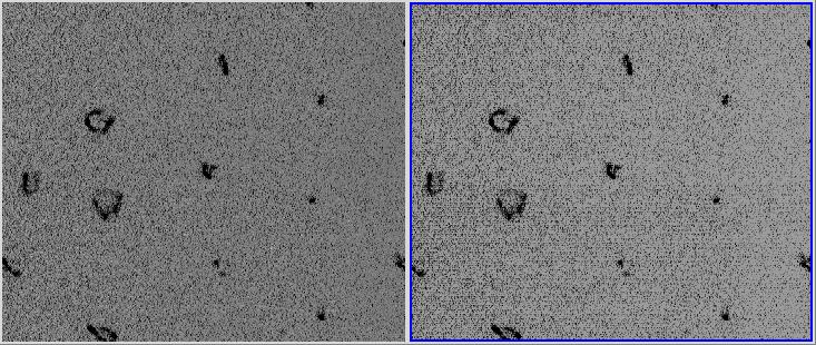Figure 0: A HEFI image treated with a bias subtraction (left) 
and without (right). The uncorrected image clearly contains 
a larger level of systematic noise. 





Step 2: Run HBTPREP
To run the HBTPREP tool, I must prepare a basic input file (called
hbtprep.in)
   # data
   final_image_name
   0
   5
   tl_f=00_h-0001.fits
   tl_f=00_h-0002.fits
   ....
The first number value after data is the focus value.  The second
value after data is the number of images in the set. This structure
is repeated enough to cover all images in the hexburst set.

A note about output names:
  To make image transfer easier, I name the stacked images with the
  follwing syntax:
    Tr_f-1200_h
  where r denotes tracker-right, and h denotes high lamp setting.
  The focus is encoded in the usual way. Canging the "t" in the
  original names to a "T" in the stacked-image names makes downstream
  data management easier.


To run the HBTPREP on your Sun or linux machine:
#  HBTPREP 
After the HBTPREP code is run, then the HBTPREP-built script named
combine.cl is run within iraf:

cl> cl < combine.cl 

This will produce the shifted HEFI images and the final composites for
each focus/tracker_state/lamp_state image set.


A SPECIAL NOTE: 
As of March 2006 I have made a number of tests with large (N=15) 
sets of HEFI images in iraf's imcombine package. Ideally, we would 
make an average stack (by setting the combine argument to "average"). 
However, occasionally we obtain corrupt HEFI image files that are 
read out improperly.  An averaging approach will suffer substantially 
from such bad images. If you use the image viewing option in HBTPREP 
to manually reject such images, then an average can be used. I suggest 
that if the completely automated approach is used (no gui reviews) then 
before you run the combine.cl script, make sure that the value of 
combine is set to "median". The median stack will be more robust 
against the occurrence of bad HEFI images. 


After combine.cl is run in iraf, the composite images are 
named comp01.fits, comp02.fits, etc. The local script (again 
built by HBTPREP) will rename the images (based on the values 
in hbtprep.in):

[sco@banzai 20050404]$ chmod 777 RENAME.scrpt
[sco@banzai 20050404]$ RENAME.scrpt

directories where 4 separate HBT runs will be performed.

At this point, if you are working on one of the Solaris machines, you might want to delete the original (unstacked) HEFI images. I usually create a subdirectory called store1, and move the stacked images (T*.fits) there. Next, you can quickly delete all files in the upper work directory. This saves valuable disk space on mcs and ion, machines that can be used to quickly reacquire the original HEFI images should you need them again.

Running HBT to Reduce the Images

The first job to do is to construct an input file (named hbt.in) that will tell HBT which images it will be processing. In addition, this file will assign a focus value to each image. An example of hbt.in is shown below:

Tl_f-1500_l.fits   1500
Tl_f-1100_l.fits   1100
Tl_f-1300_l.fits   1300
Tl_f-1700_l.fits   1700
Tl_f-1900_l.fits   1900
Tl_f-2100_l.fits   2100 
Tl_f-2300_l.fits   2300 
Tl_f-900_l.fits     900 

The format of hbt.in is pretty simple. Each line in the file corresponds to a different image. On each line (in free format) we list the image name and the focus seeting used to generate that image. The focus values must be entered as integer values (i.e. use 2300 instead of 2300.0). You can generate this file using any kind of editor (like vi or emacs).

A useful thing to know prior to running HBT is that sometimes you will be asked if you want to skip a step or skip to another section of the code. These are shortcut steps that can be performed only if previous HBT runs on your data have been made. In general your answer will be N . Actually, you can also just enter a return and HBT will know not to make the skip.

[sco@banzai TL_l_jun16_raw]$  HBT 
Assumed platform = del

Number of hex-burst images =  8

Skip opening a ds9 window? (Y/N):  N  

Jump directly to combine and analysis? (Y/N):  N 

Jump directly to HBT-related tasks? (Y/N):   N  

Enter desired thresh,irad,ism (3.0,10,2):  5 10 2 

At this stage, the program is preparing to detect the mirror sources in your firts HEFI image. You must supply the detection parameters for this. The last 3 numbers above (5 10 2) are values that I have found to be good values for our hexburst images thus far. After you enter these values, the sources are located and an image much like what you see in Figure 1 is displayed. The only difference is that you must interactively draw the blu line in the ds9 gui that locates the central column of the HET mirror array. The line marker is already set be a "BLUE LINE". You simply click on the top mirror position and drag to the bottom mirror position. Note that before doing this, it is often convenient to use the "Zoom to Fit Frame" option in the Zoom menu, so that the entire HEFI image is visible.

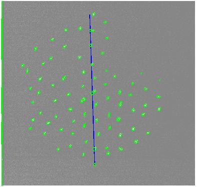Figure 1: A typical HEFI image of the HET mosaic obtained during a hexburst. The individual mirror images (the white spots) have been located with a source-finding code (SExtractor) and circled with green ellipse markers. In order to begin the process of identifying mirrors, we must give HBT an idea of the location and size of the central column of mirrors. We set this location graphically in a ds9 window (opened by the code) with a blue line marker. We place the top part of the line segment on the top mirror (6:11) and the bottom part of the line segment on the bottom mirror (6:1).

Once the central column of mirrors has been located, HBT will have an estimate of the location, orientation and scale size of the HET mirror array on the HEFI image. At this point, you may wish to identify mirrors that are clear problem cases. You can do this using different ds9 marker symbols, as is outlined in the HBT command window at this point in running the code. An example of this is shown in Figure 2.

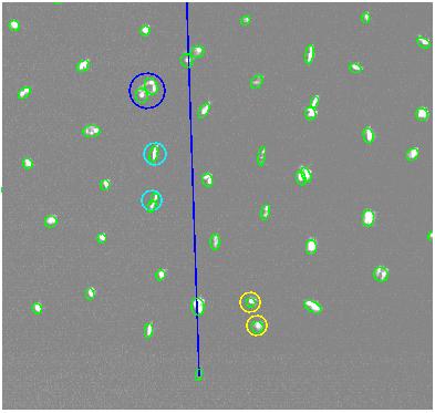Figure 2: An example of identifying special mirror cases with a ds9 marker. This step is optional now, but may someday a very important part of the HBT reduction. As the HBT command window will tell you, we use (1) YELLOW circles to locate images from different mirrors that are very close together. (2) BLUE circles to identify a doughnut mirror (3) CYAN circles to identify an astigmatic mirror. After you hit a return in your ds9 window, HBT will paint up the assumed positions for the HET mirrors using cyan hexagons.

When you hit a return in the HBT command window, whether or not you have marked problem mirrors, the program will next paint up the HEFI image, along with a set of cyan hexagons that denote where each HET mirror is presently thought to be located. An example of this is shown in Figure3. Note also that you see sets of red circles also drawn. These red circles indicate the actual locations of the mirror images that HBT has adopted for each source. Close inspection of Figure 3 reveals that a number of the "sources" in the image are actually composed of several green ellipse markers (i.e. multiple detections were obtained in the source detection phase). The red circles indicate how sets of multiple detections for a single source are "glued" together to represent one mirror image. The next thing you should notice in Figure 3 is that many of the mirror positions (the red circle positions) do not sit in the middle of their respective cyan hexagons. In other words, HBT does not yet have a good value for where these mirror images are really located. Hence, we must communicate a revised position, or offset position, for those mirrors that are not located well. The yellow line marker that you see in Figure 3 accomplish this. For each badly located mirror, you just click in the approximate center of the appropriate cyan hexagon, and then drag to the appropriate mirror (red circle) image. After this you will see a yellow line indicating the offset you have just set.

Presently, I prefer to mark a yellow offset line for nearly every mirror source in this firt HEFI image. HBT will use these offsets in all subsequent images as a first guess to where each image should be. Since we are only change the focus position in each image, and no actual mirror offsets (i.e. actuator adjustements) have been applied, then these relative mirror offset positions should sclae with the size and location of the HET array on each HEFI image.

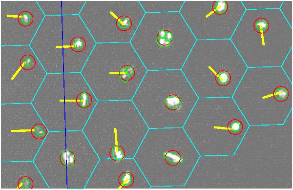Figure 3: A close up view of the HET mirror positions currently assumed by HBT. The assumed mirror positions are painted up as cyan hexagons. Use the YELLOW line marker to correct the positions of badly positioned mirrors. Attach the initial line endpoint to the approximate center of the correct cyan hexagon, and connect the final line endpoint to the red-circled image for the mirror you wish to identify.

After you hit a return in the HBT command window, a new image like that in Figure 4 is drawn. This shows which mirror sources you have drawn offsets for.

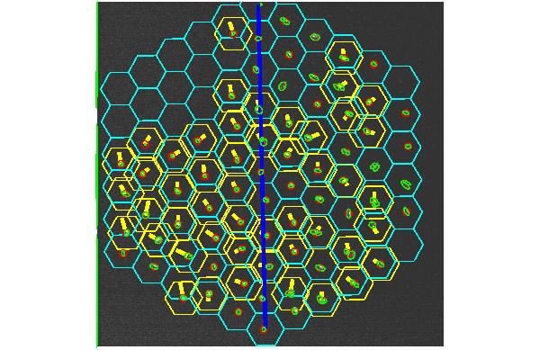Figure 4: After setting the yellow line segments, and hitting a return in the HBT command window, you will a graphic such as this. For every mirrror that you assigned an offset, that new position will be indicated by a yellow hexagon.

After you hit a return in the HBT command window, a new image like that in Figure 5 is drawn. This shows the current state of mirror offsets you have adopted for this HEFI image. You can apply more yellow line segments at this stage, but by the time you get here (for each HEFI image) you are done.

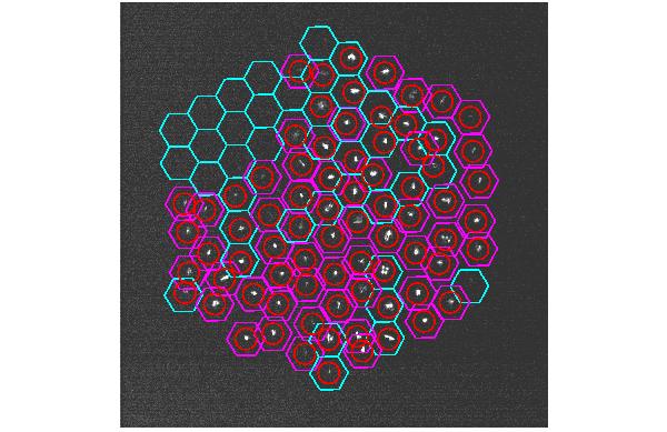Figure 5: After hitting a second return in the HBT command window, you will a graphic such as this. It is basicaly a less complicated version of Figure 4. All mirrors with special offset positions are painted with magenta hexagons, and those with no offset are painted as the usual cyan hexagon. At this point, you may once again use the yellow line marker to assign offsets. You can do this for either type of hexagon (cyan or magenta). You enter a return in the HBT command window when you are satisfied with your updated positions (if you entered any).

At this stage, the process is repeated for the next (and all subsequent) images that you have listed in the hbt.in file. You'll once again have to mark the position and size of the central mirror column. However, after the central column is marked in these subsequent images, you will see that the mirror positions are painted onto the screen with the special offsets set in your first image, but appropriately scaled to match the scale size of the current HEFI image. If all is well, you should not have to use any yellow line segments to re-position mirrors.

A special case of HEFI image

In the more extreme focus positions, the array of mirror images will overflow the field of view of the HEFI image. Unfortunately, this means that we may be unable to locate mirrors 6:1 and 6:11 (the top and bottom mirrors in the HET array). The solution is it locate other mirrors in the central column. The logical choices are 6:2 and 6:10. We do this by changing the line marker color from blue to red when we are asked to mark the central column. After this is done, and the program recognizes a red line has been used, you will be queried for the actual mirror numbers you have used. These will almot always be 10 for the top and 2 for the bottom, but you have the capabilitu of using any mirrors in the central column.

Finishing the Job: The Old Pre-Spring06 Method

Currently, much of the analysis described in this section is performed by stand-alone downstream codes. For completeness, and because we can still use HBT alone for the anlysis, I am retaining this description of the old approach in the manual.

At this stage in the HBT execution, we have located our mirrors, and computed image parameters for each mirror in each focus position. We'll now determine which HEFI image provides the best focus image for each identified mirror.

 
Skip the combine and webpage steps? (Y/N): N  
Graphically review focus curve fits? (Y/N): Y

After you answer the last question above, a fairly long process will occur: a small image around each mirror, in each HEFI image, is extracted and archived for later use. These "postage stamp" images will be used for later photometric parameter determination and web-based image graphicster on. This last query above concerns how we will select the best focus position for each mirror. If you answer Y (which is what we'll generally alway do), then HBT will beging to exhibit the focus curve for each mirror. A PGPLOT window will appear that shows, for each mirror, a plot of R50 (Y axis) versus focus position (X axis). The parameter R50 is the radius of a circle (in arcsecond units) that encloses half the total light in a mirror image. Hence, at best focus, this value should be at a minimum. In reality, there are a host of problems that can occur in computing R50 (and everything else!) that can occasionaly produce a spuriosly low value of R50. Hence, we will use the focus plots to eliminate such cases. We can use the stamp images painted in the ds9 window to help judge proble cases. The image associated with each point in our focus plot is shown in the ds9 window. The focus value is printed in read letters in the bottom left-hand corner of each stamp.

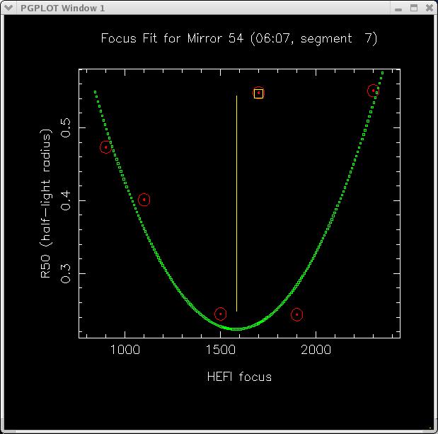Figure 6: A focus plot used in HBT to determine best focus position. Obviously discrepant data points can be rejected with the "Z" key, and are painted with a yellow box. If desired, a parabolic fit can be computed with the unrejected points with the "P" key. The resultant parabola (shown in green above) is used to estimate the best focus position for this mirror.

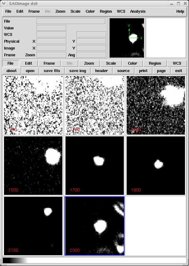Figure 7: The postage images associated with each point in the focus plot of Figure 6.

After the last focus plot is inspected (usually somewhere close to segment #91), the HBT program will collect all best focus positions and and construct a web document that summarizes the results of the analysis. This document resides in a local subdirectory named "web".

Running HBTFINAL

HBTFINAL is used to stack individual mirror images for each focus set. The stacked stamp images are stored in the local directory (created by HBTFINAL) called stamps_1. When the stamps are cut, they are then photometered. The results are stored in the HBTFINAL-created directory called mirror_data. After the stamps are photometered, the user interactively fits focus curves for each mirror set. Currently, the final results of this analysis are written to a file called "list_1.out".

Running HBTWEB

HBTWEB is run in the top level directory of you hexburst reduction directory (i.e in ~sco/hex_real/20070617). It creates a local web directory with a set of html documents that summarize the reduction and allow the user to quickly see the summary plots for each mirror in the analysis. The name of the directory is web_DATE, where DATE is the name of the reduction directory (i.e. 20070617). These are stand-alone directory trees that can be easily transfered to the hexburst data home page.

Running REFOC

In some cases, usually due to user error, the hexburst focus curve for a mirror may have been fitted incorrectly. You can use the REFOC code to refit single mirrors. This code is run in the top-level redcution directory (just like HBTWEB). You must run it once for each mirror to be corrected. In esseance, this code reconstructs the plots focus_r50.gif and profile.gif in the mirror_data/hex** subdirectroies. It also reconstructs the files recording information about the selected best-focus image.

It is important to remeber that after you use REFOC, you must re-run the HBTWEB tool in order for the changes to be made in the summary web page.