Tutorial
Did you read the Introduction? Did you read about the Classes? You really should! But then again, nobody does. Also it really helps to know a bit about Python as well as Numpy and Matplotlib. But to heck with that. Who reads manuals anyway. Let’s get started because this is really the fun part.
Start by launching Python and importing the necessary packages.
import matplotlib.pyplot as plt
import numpy as np
from sas import amslog as sl
I hope you know where the Sams logs files are kept because we will need to access them. At the Het they can be found in /home/jove/guider/SAMS/7.1/archive. I’m just going to use the file names but you may have to prepend an absolute or relative directory to the names in order to get access to it. Let’s create our first Sams Log object.
sen = sl.SamsLog(['sams201708130000.sen'])
Note that you could have listed the five other files to get a full days worth of data or you can use the day prefix as a short cut. For example, you could use this form to get all the files.
sen = sl.SamsLog(['sams20170813'], suffix='sen', verbose=True)
Reading file sams201708130000.sen   in 2.734 seconds
Reading file sams201708130400.sen   in 12.328 seconds
Reading file sams201708130800.sen   in 3.099 seconds
File "sams201708131200.sen" does not exist
File "sams201708131600.sen" does not exist
File "sams201708132000.sen" does not exist
Converting time   in 0.286 seconds

sen.files()
['sams201708130000.sen', 'sams201708130400.sen', 'sams201708130800.sen']
Refer to the samslog.py for more information.
You can find out what type of data are in the object as well as the size of the data.
sen.suffix()
'sen'
sen.size()
(26480, 481)
The first value (26480) is the number of rows and the second value (481) is the number of columns. Remember that there is a date/time stamp at the start of each row so with 480 sensors that makes 481 columns.
So let’s plot some values. These commands will create the following plot.
tstamp, sen1, sen2, sen3, sen4, sen5, sen6 = sen.data('M43')
plt.plot(tstamp, sen1, 'r', legend='M43-1')
plt.plot(tstamp, sen2, 'g', legend='M43-2')
plt.legend()
plt.show()
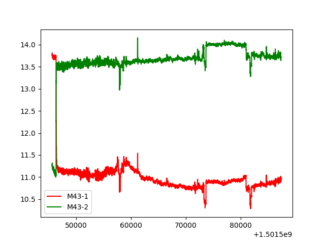
Sensor 1 and 2 plots for segment M43
If you ask for an edge segment, then None will be returned as the values for that particular sensor data. You should test for this before naively plotting these data.
Similarly you could look at Tip/Tilt data for the same period.
ttp = sl.SamsLog(['sams20170813'], suffix='ttp')
ttpstamp, m43tip, m43tilt, m43pist = ttp.data('M43')
plt.plot(ttpstamp, m43tip, 'r', label='M43 Tip')
plt.plot(ttpstamp, m43tilt, 'g', label='M43 Tilt')
plt.ylim(-0.1, 0.1)
plt.legend()
plot.show()
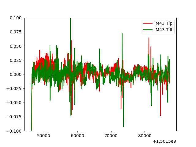
Tip and tilt plotted for Segment M43
Or you could look at the tip/tilt data as a summary plot.
plt.quiver(np.zeros_like(m43tip), np.zeros_like(m43tilt), m43tip, m43tilt)
plt.show()
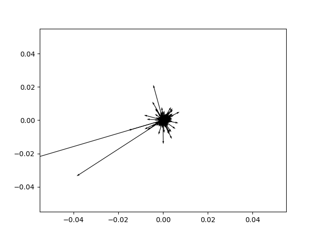
All the tip/tilts from segment M43 plotted as vectors
If you want to get even fancier, it is possible to plot an entire nights tip/tilt data for the entire array.
ttp = sl.SamsLog(['./data/sams20170813'], suffix='ttp', verbose=True)
plot_ttp_summary(ttp)
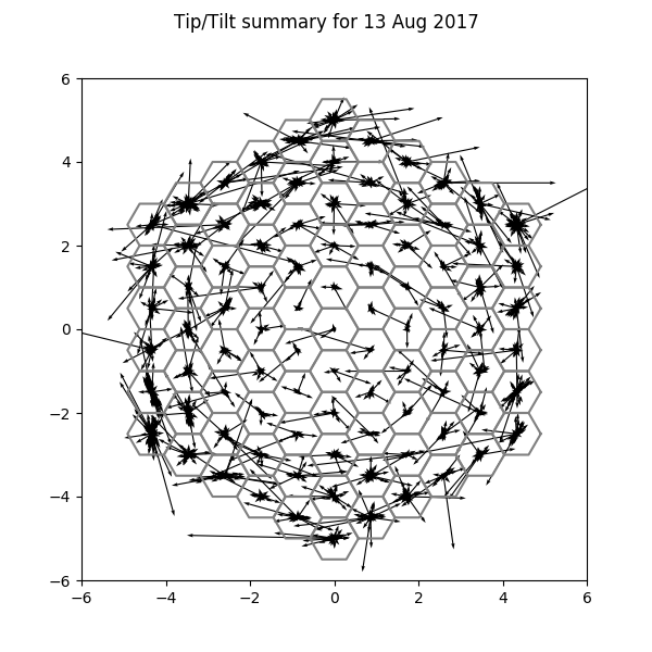
The tip/tilt data for all segments.
The summary files contain global and average information for the time period. You can make a summary plot with the command plot_sum_summary().
sum = sl.SamsLog(['./data/sams20170813'], suffix='sum', verbose=True)
plot_sum_summary(sum)
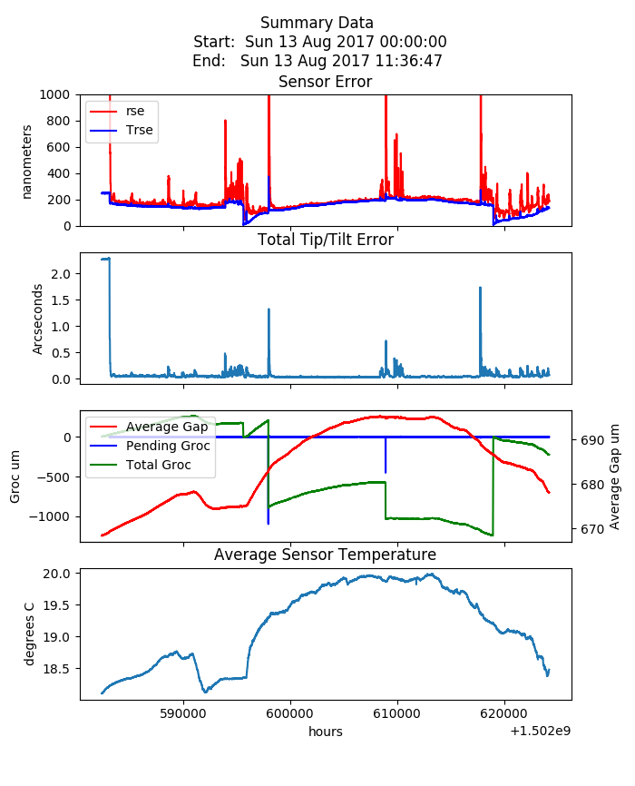
The summary plot of global and average values.
Numerous possibilities are open to you. You just need to use your imagination.